This post aims to summarize the main concepts involved in a symbol timing synchronization scheme by exploring a MATLAB example. For the reader interested in going deeper into the topic, I recommend Michael Rice’s digital communications book [1], which is the book referenced by MATLAB’s symbol timing synchronization implementation. Finally, after understanding the concepts presented there, I recommend exploring the MATLAB simulation that I developed and published on Github:
https://github.com/igorauad/symbol_timing_sync
Contents
- 1 Background
- 2 Pulse Shaping Filter Design Considerations
- 3 Transmitter
- 4 Channel
- 5 Receiver without Symbol Timing Synchronization
- 6 Receiver with Symbol Timing Synchronization
- 7 Derivative Matched Filter (dMF)
- 8 dMF design
- 9 Maximum likelihood Timing Error Detector (ML-TED)
- 10 Zero-crossing Timing Error Detector (ZC-TED)
- 11 Final Remarks
- 12 References
Background
What is symbol timing synchronization?
Since there are many flavors of synchronization, the precise definition of each synchronization can become confusing. For example, there is clock synchronization, frame synchronization, carrier synchronization, all of which are different concepts than symbol timing synchronization.
Symbol timing synchronization has a unique purpose: to find the optimal instants when downsampling a sequence of samples into a series of symbols. In other words, it focuses on selecting the “best” sample out of every group of samples, such that this selected sample can better represent the transmitted symbol. The chosen sample (deemed as the symbol) is then passed on to the symbol detector. This concept will become clear once we explore a couple of examples.
Components of a Symbol Timing Recovery Loop
At this point, it is instructive to revisit what a basic feedback control loop is. In essence, a control loop has three main elements: an error detector, a filter, and a “plant” (or “process”). Its goal is to control the response produced by a particular input signal. For example, when a power switch is turned on (say from 0 to 12V), a control loop can control the pace at which the output voltage transitions from 0 to 12V, for example, by guaranteeing that it settles at 12V steadily within a given time specification. The error detector compares the input and the output of the loop. The difference (the detected error) is filtered by a block known as the “controller.” This controller has several parameters capable of controlling the desired output response (for example, the just mentioned settling time). Finally, the filter output feeds the “plant,” which generates a signal following the input. The error decreases as the plant’s output approaches the input signal. Ultimately, after enough time, the system converges to its steady state.
Timing recovery loops are just that, but with their peculiar error detector, filter and plant. In the sequel, you can find a very brief overview of the timing recovery loop elements. Do not worry if their essence is not clear yet. It will soon be once we advance into the MATLAB examples.
Timing Error Detector
First, note the n-th receive symbol can be modeled by:
\(y(nT_s) = \sum \limits_{m}x(m)p((n-m)T_s – \tau) + v(nT_s), \)
where \(T_s\) is the symbol period, \(p\) is the channel pulse response (combining both the pulse shaping filter and the receiver-side matched filter), \(x(m)\) is the m-th transmit symbol, \(v(nT_s)\) is the AWGN and, importantly, \(\tau\) is the timing offset error within \([0, T_s)\), that is, within a fraction of the symbol period.
The timing offset error \(\tau\) results from the channel propagation delay, which can not be controlled and, therefore, introduces delays that are not simply integer multiples of the symbol period. In reality, the propagation delay is such that \(\tau\) is composed of two terms: an integer and a fractional multiple of \(T_s\). In the context of symbol timing recovery, we are only concerned with the fractional error. The integer error is handled by a frame timing recovery (or frame synchronization) scheme.
Since the pulse \(p(t)\) is designed for zero intersymbol interference (ISI), it is only because of the timing error \(\tau\) that the terms for \(n \neq m\) in the summation of the above expression for \(y(nT_s)\) are non-zero. As a result, due to \(\tau\), the received symbol \(y(nT_s)\) is corrupted by both AWGN and ISI.
The timing error detector has the purpose of estimating this timing error \(\tau\), so that the receiver can adjust its timing and avoid the intersymbol interference.
Loop Filter
The loop filter controls how fast the timing error can be corrected, what types of errors can be treated (for example, linearly varying), and the range of correctable timing errors. In general, it is a second-order system and often the proportional-plus-integral controller (PI controller), commonly used in feedback systems. In this post, we choose not to give in-depth details about the loop filter. Instead, the reader may find a comprehensive discussion in [1] (see Appendix C).
Interpolator Controller and Interpolator
Finally, the interpolator and the interpolator controller in conjunction represent the plant (or process) in the context of symbol timing recovery. The interpolator controller chooses the samples of the matched-filter output sequence to be retained as the symbols. For an oversampling factor of \(L\), the MF outputs \(L\) samples for each symbol. In turn, the receiver has to pick only one out of each \(L\) and pass it to the symbol detector. Hence, it is as if the interpolator controller generated a train of spaced impulses, with impulses solely at the indexes corresponding to the desired symbols.
This tutorial does not discuss the interpolator and its controller. So, again, the reader is referred to [1].
In the end, a timing recovery loop generally looks similar to the following diagram:
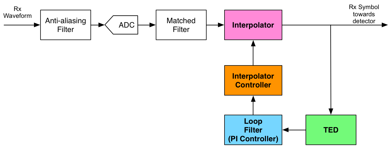
With that, we are ready to advance to the tutorial. By looking into MATLAB code and corresponding plots, the main aspects of the timing recovery loop will become clear.
Pulse Shaping Filter Design Considerations
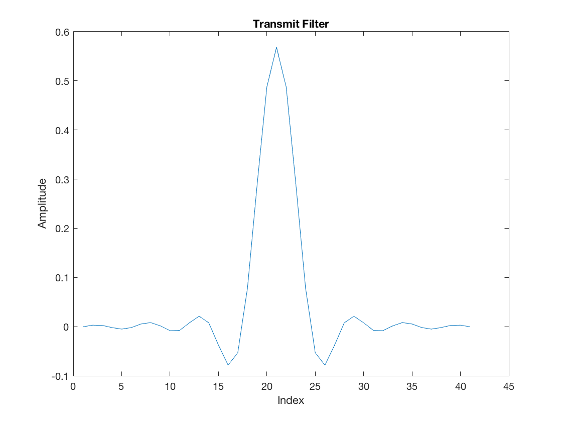
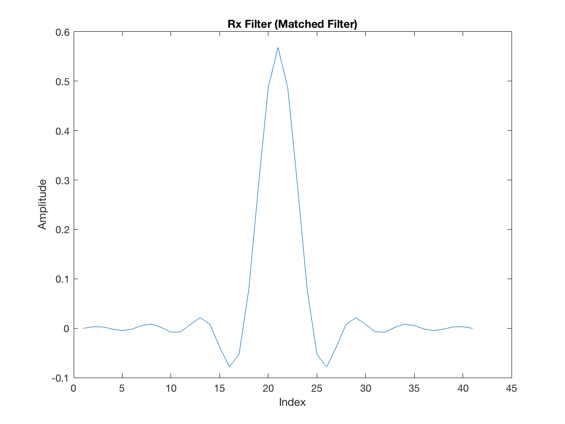
First, design a Square-root Raised Cosine filter for pulse shaping:
L        = 4;         % Oversampling factor
rollOff  = 0.5;       % Pulse shaping roll-off factor
rcDelay  = 10;        % Raised cosine delay in symbols

% Filter:
htx = rcosine(1, L, 'sqrt', rollOff, rcDelay/2);
% Note half of the target delay is used, because when combined
% to the matched filter, the total delay will be achieved.
hrx  = conj(fliplr(htx));

figure
plot(htx)
title('Transmit Filter')
xlabel('Index')
ylabel('Amplitude')

figure
plot(hrx)
title('Rx Filter (Matched Filter)')
xlabel('Index')
ylabel('Amplitude')

p = conv(htx,hrx);

figure
plot(p)
title('Combined Tx-Rx = Raised Cosine')
xlabel('Index')
ylabel('Amplitude')

% And let's highlight the zero-crossings
zeroCrossings = NaN*ones(size(p));
zeroCrossings(1:L:end) = 0;
zeroCrossings((rcDelay)*L + 1) = NaN; % Except for the central index
hold on
plot(zeroCrossings, 'o')
legend('RC Pulse', 'Zero Crossings')
hold off

The zero-crossings highlighted in the RC pulse are very important in the context of symbol timing synchronization. Once the receiver samples the incoming waveform and performs matched-filtering, the samples retained as symbols must be aligned with these zero-crossings. If that is guaranteed, the intersymbol interference is eliminated. In other words, a given symbol is multiplied by the RC peak (unitary in this case), and its interference contribution to all other neighbor symbols is exactly the amplitude at the zero-crossings, namely null.
Transmitter
Next, observe the transmission of a 2-PAM symbol sequence. Let’s say we transmit a couple of consecutive PAM symbols over a period that at least is longer than the RC delay:
M = 2; % PAM Order

% Arbitrary binary sequence alternating between 0 and 1
data = zeros(1, 2*rcDelay);
data(1:2:end) = 1;

% PAM-modulated symbols:
txSym = real(pammod(data, M));

figure
stem(txSym)
title('Symbol Sequence')
xlabel('Symbol Index')
ylabel('Amplitude')
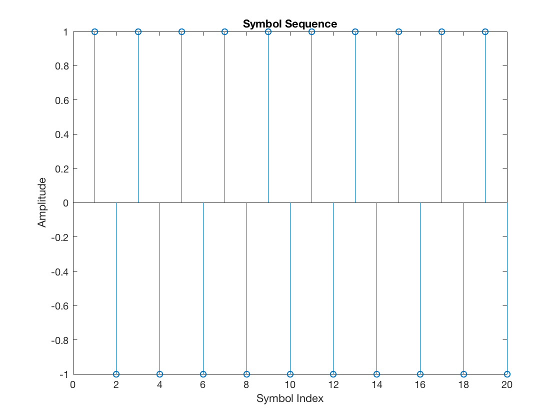
Note we intentionally generated the sequence with alternating +1, -1, +1, -1, and so forth. First, this will help with visualization. Secondly, and more importantly, this property will be critical when we discuss a specific timing error detector scheme. Keep that in mind.
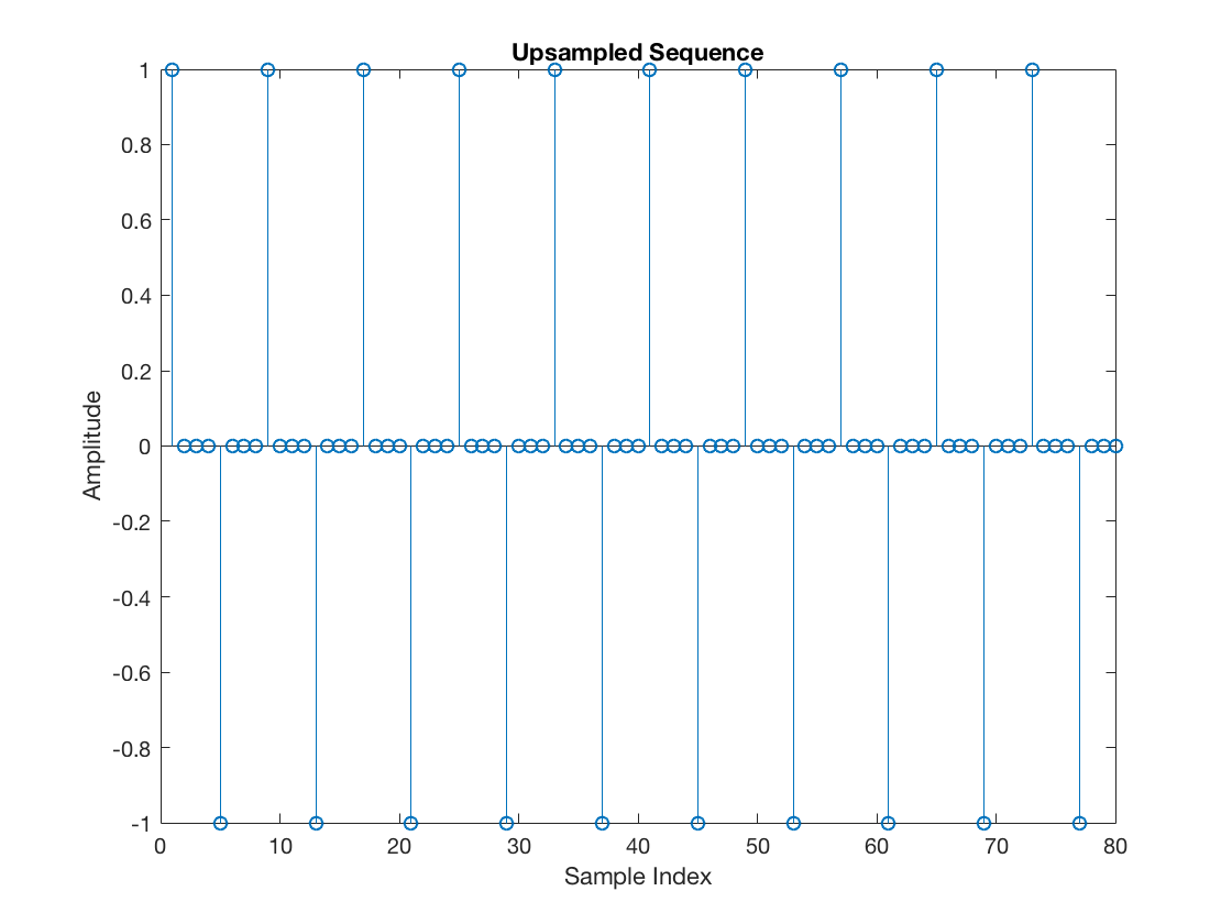
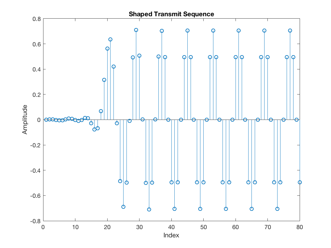
% Upsampling
txUpSequence = upsample(txSym, L);

figure
stem(txUpSequence)
title('Upsampled Sequence')
xlabel('Sample Index')
ylabel('Amplitude')

% Pulse Shaping
txSequence = filter(htx, 1, txUpSequence);

figure
stem(txSequence)
title('Shaped Transmit Sequence')
xlabel('Index')
ylabel('Amplitude')
Channel
Next, let’s add a random channel propagation delay in units of sampling intervals (not symbol intervals):
timeOffset = 1; % Delay (in samples) added

% Delayed sequence
rxDelayed = [zeros(1, timeOffset), txSequence(1:end-timeOffset)];
Furthermore, let’s completely ignore AWG noise. This simplification will make the symbol timing synchronization results more apparent and help the explanation.
Receiver without Symbol Timing Synchronization
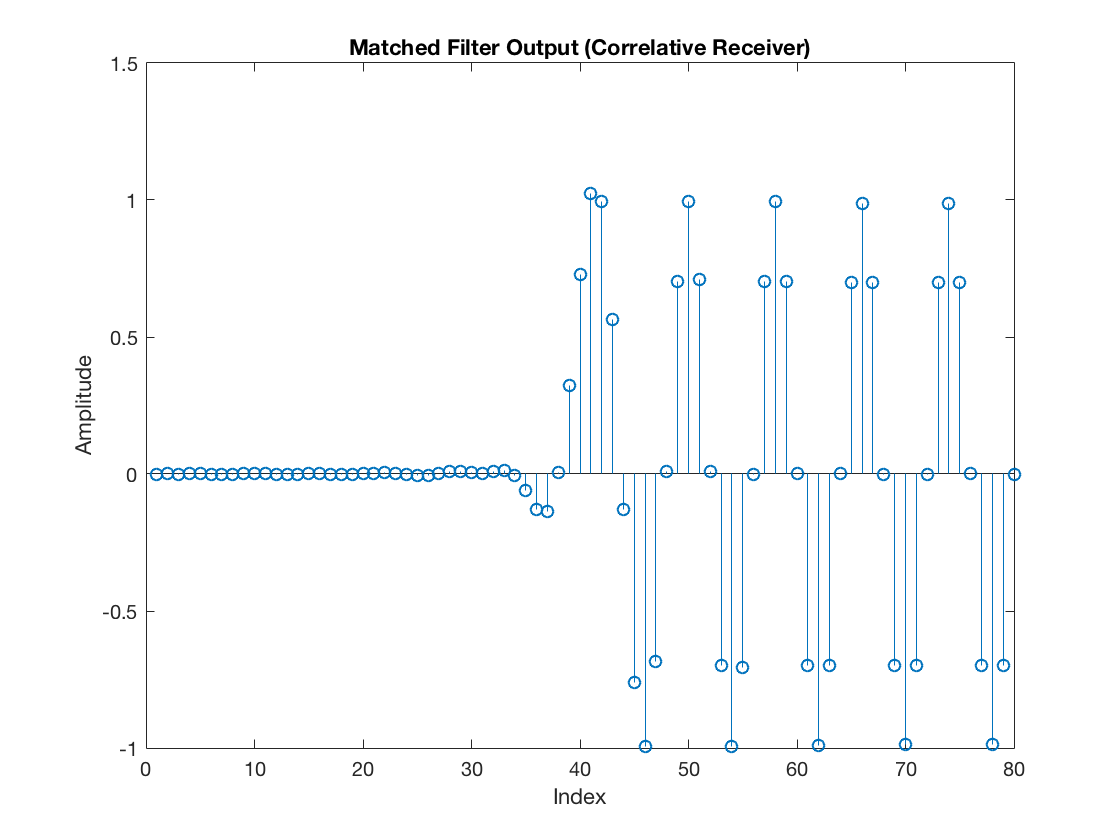
Now, let’s consider a receiver that does not perform symbol timing synchronization. As the initial block diagram illustrates, assume the matched filter block precedes the symbol timing recovery loop. Hence, apply the matched filtering first, as follows:
mfOutput = filter(hrx, 1, rxDelayed); % Matched filter output

figure
stem(mfOutput)
title('Matched Filter Output (Correlative Receiver)')
xlabel('Index')
ylabel('Amplitude')
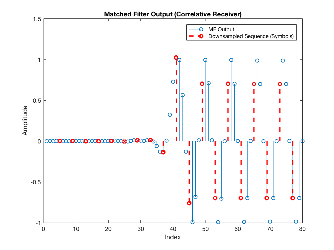
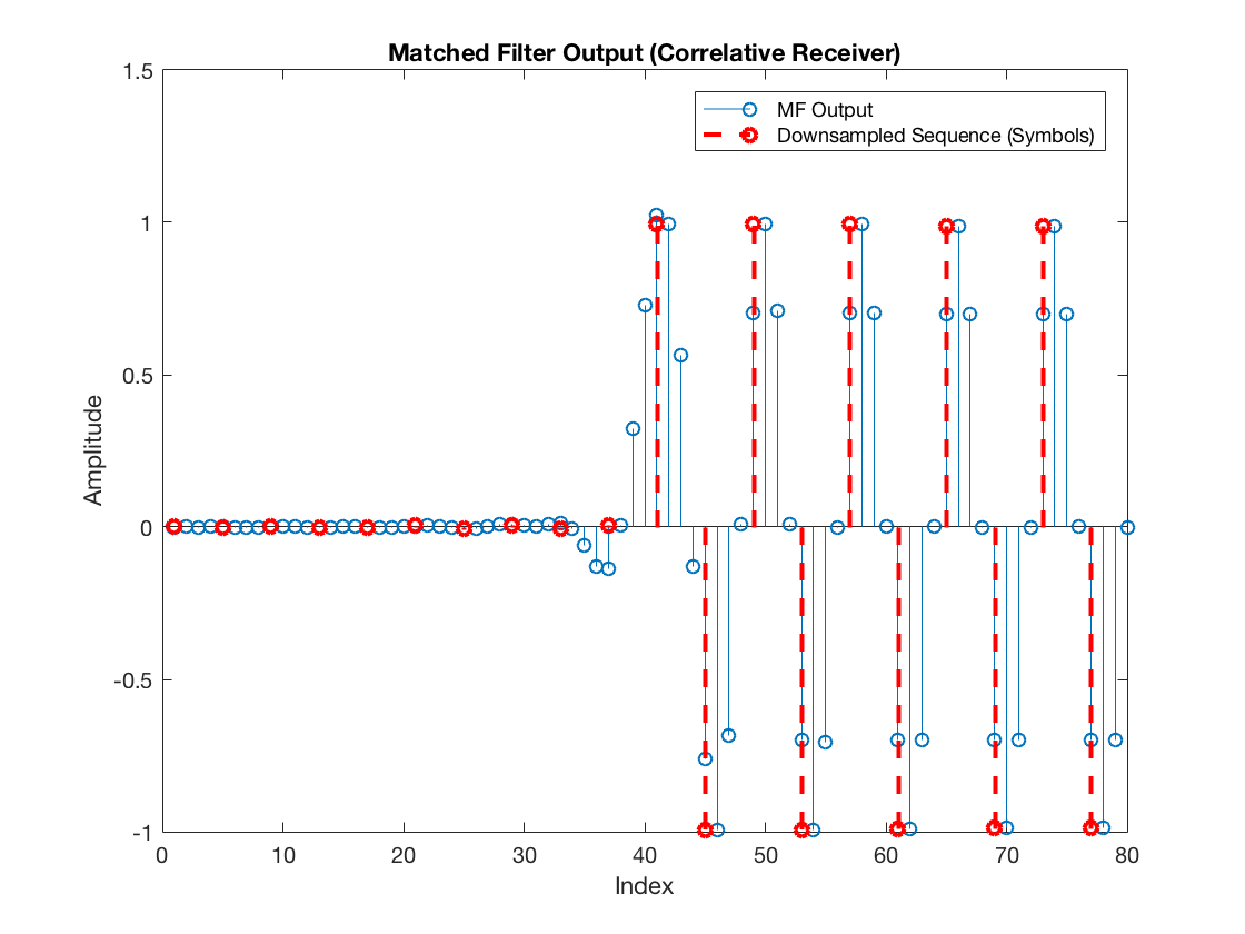
Next, let’s add an arbitrary timing used by the receiver to select samples from the incoming sequence and pass them to the decision module (namely for the downsampler).
rxSym = downsample(mfOutput, L);

% Generate a vector that shows the selected samples
selectedSamples = upsample(rxSym, L);
selectedSamples(selectedSamples == 0) = NaN;

% And just for illustration purposes
figure
stem(mfOutput)
hold on
stem(selectedSamples, '--r', 'LineWidth', 2)
title('Matched Filter Output (Correlative Receiver)')
xlabel('Index')
ylabel('Amplitude')
legend('MF Output', 'Downsampled Sequence (Symbols)')
hold off
In this case, the extracted samples (the received symbols) look as follows:
figure
stem(rxSym)
title('Symbol Sequence')
xlabel('Symbol Index')
ylabel('Amplitude')
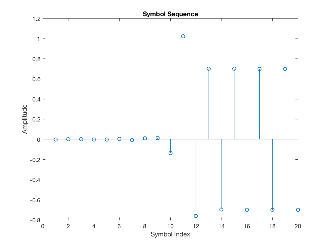
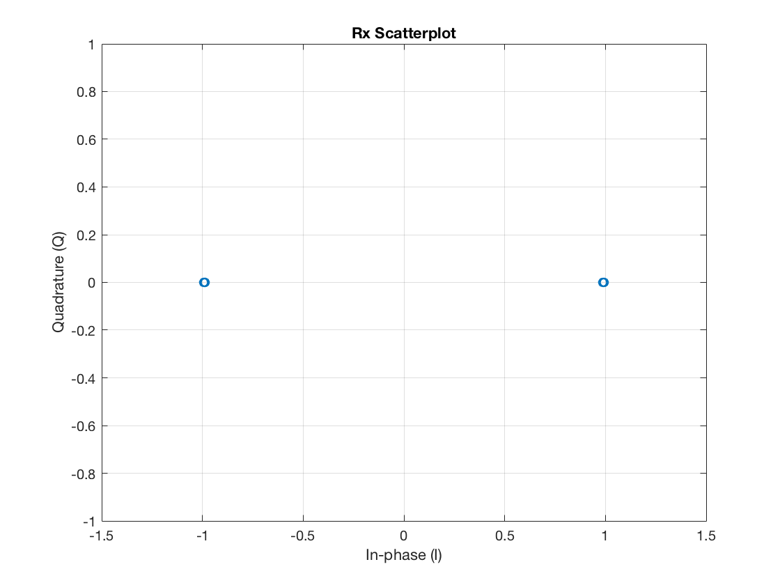
Finally, after skipping the transitory due to the raised cosine pulse delay, the corresponding scatter plot becomes:
figure
plot(complex(rxSym(rcDelay+1:end)), 'o')
grid on
xlim([-1.5 1.5])
title('Rx Scatterplot')
xlabel('In-phase (I)')
ylabel('Quadrature (Q)')
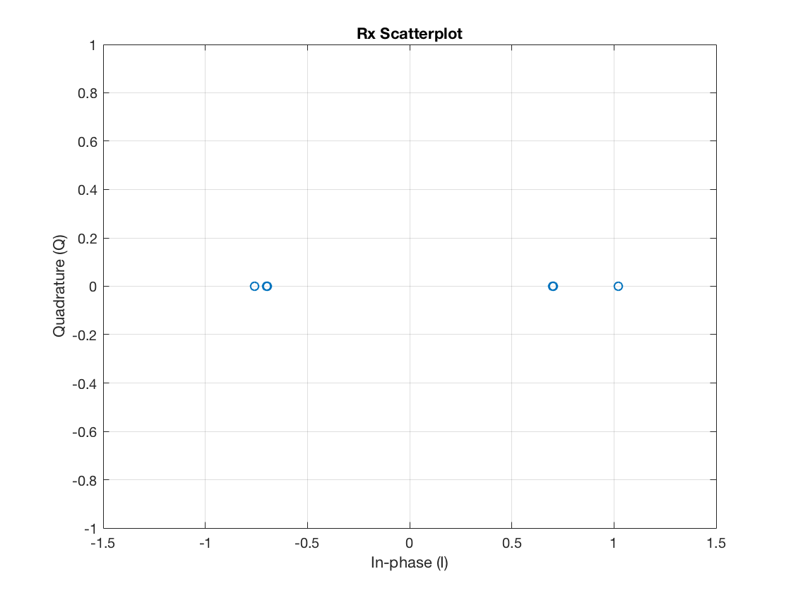
Note it is not looking good enough yet. The receiver is not extracting the samples aligned with the zero-crossings of the pulse shaping function. Consequently, the retained symbols are disturbed by intersymbol interference.
Receiver with Symbol Timing Synchronization
Now let’s suppose the receiver knows the symbol timing offset exactly, in terms of sampling periods or, equivalently, fractional symbol intervals. Let’s add the timeOffset variable to the offset argument of the downsample function:
rxSym = downsample(mfOutput, L, timeOffset);
In this case, we can see that the “selected” samples are:
selectedSamples = upsample(rxSym, L);
selectedSamples(selectedSamples == 0) = NaN;

figure
stem(mfOutput)
hold on
stem(selectedSamples, '--r', 'LineWidth', 2)
title('Matched Filter Output (Correlative Receiver)')
xlabel('Index')
ylabel('Amplitude')
legend('MF Output', 'Downsampled Sequence (Symbols)')
hold off
Hence, the symbols passed to the PAM decision module are:
figure
stem(rxSym)
title('Symbol Sequence')
xlabel('Symbol Index')
ylabel('Amplitude')
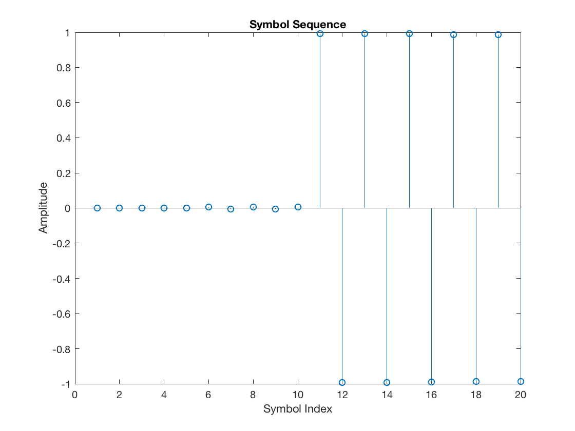
And, again, skipping the raised cosine pulse delay, the symbol scatter plot becomes:
figure
plot(complex(rxSym(rcDelay+1:end)), 'o')
grid on
xlim([-1.5 1.5])
title('Rx Scatterplot')
xlabel('In-phase (I)')
ylabel('Quadrature (Q)')
Perfect, isn’t it? So, in conclusion, all the receiver needs is to find somehow the exact instants of the zero-crossings within the time-shifted pulse shaping functions representing each transmitted symbol. This task is supported by the timing error detector (TED) of the symbol timing recovery loop. In particular, the TED aims to indicate how well the current symbol timing alignment is relative to the zero crossings. We discuss two possible TED approaches next.
Derivative Matched Filter (dMF)
One of the possible TED schemes is the so-called maximum likelihood TED (ML-TED). It employs a derivative matched filter (dMF), which, as the name implies, is a filter whose output corresponds to the derivative of the matched filter. The idea is that the MF derivative approaches zero whenever the MF response reaches a peak, i.e., when its slope transitions from positive to negative. Let’s see how this looks like in practice.
First, let’s design the dMF. Before doing so, note there are several ways of approximating a derivative in discrete time. The main distinction lies in the resulting frequency response of the filter and, more specifically, how the filter deals with noise. An approach that avoids enhancing high-frequency noise is the central differences differentiator (refer to this informative post). Therefore, we choose this approach in what follows:
dMF design
h = [0.5 0 -0.5]; % central-differences kernel function
central_diff_mf = conv(h, hrx);

% Skip the kernel delay
dmf = central_diff_mf(2:1+length(hrx));

figure
plot(hrx)
hold on, grid on
plot(dmf, 'r')
legend('MF', 'dMF')
title('MF vs. dMF')
xlabel('Index')
ylabel('Amplitude')
hold off
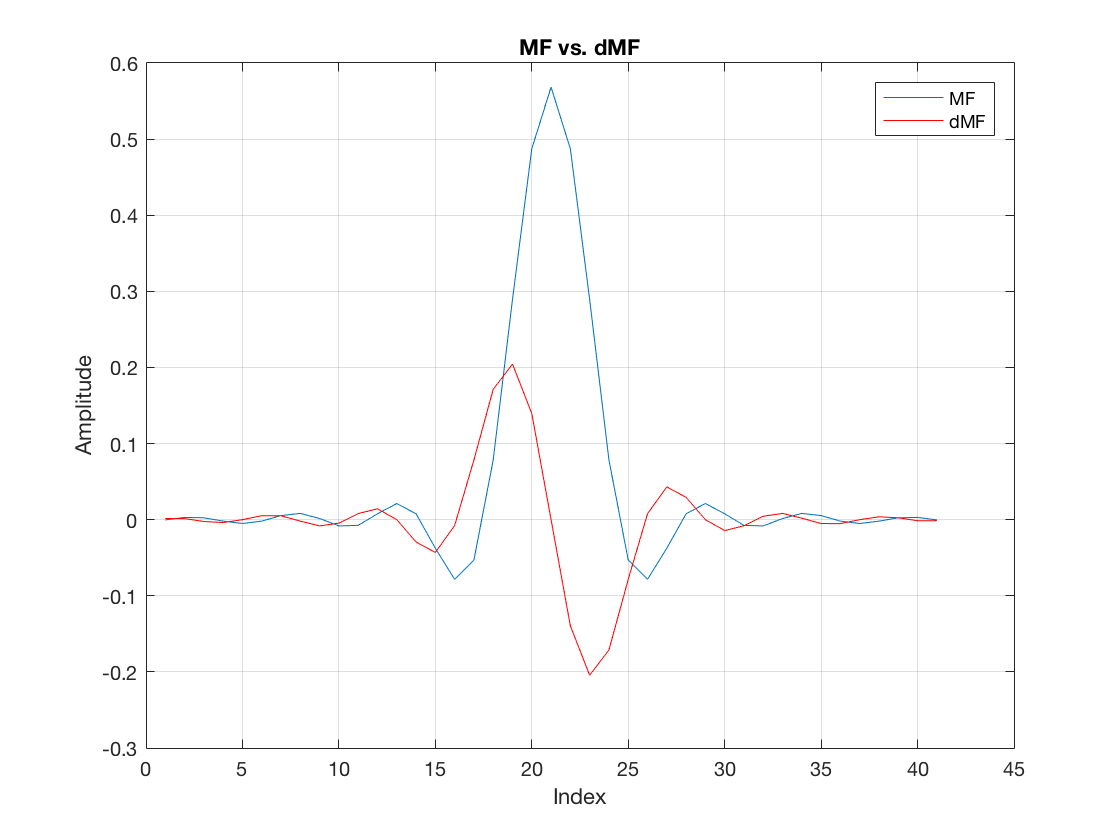
So, as expected, we can see that the very center of the MF (the peak) is aligned with a zero amplitude at the dMF. Hence, the dMF can provide a good indication as to whether the receiver is correctly observing the MF peak. That is, the dMF output should be roughly zero at this point.
Nevertheless, it is worth clarifying that the dMF is designed to indicate the peaks associated with each time-shifted RC pulse (due to each transmitted symbol), not the peak values observed in the combined MF output. Recall from the model of \(y(nTs)\) presented in the beginning that the n-th received symbol is a sum of time-shifted pulses (i.e., time-shifted RC pulses). Furthermore, recall that the RC pulse is designed for zero intersymbol interference at the suitable locations (the symbol instants) but does not guarantee zero interference elsewhere. Hence, when you look at the sum of pulses forming \(y(nTs)\), the correct symbol instants are not on the peak values. In contrast, when looking at the individual RC pulses generated by each transmitted symbol, the right symbol location coincides with the peak of the individual pulses. You can observe this better by playing with the following snippet on your own:
N = 5; % Symbols to observe
rndData = randi(M, 1, N) - 1; % Random data
rndTxSym = real(pammod(rndData, M)); % Tx symbols
rcLen = 2*rcDelay*L + 1; % RC pulse length
mfOutLen = rcLen + N*L - 1; % MF output length
mfOutMtx = zeros(N, mfOutLen); % Individual MF responses
dmfOutMtx = zeros(N, mfOutLen); % Individual dMF responses
selectedSamples = NaN * ones(1, mfOutLen);

for i = 1:N
    txSymInd = zeros(1, N);
    txSymInd(i) = rndTxSym(i);
    txSeq = conv(htx, upsample(txSymInd, L));
    mfOutMtx(i, :) = conv(hrx, txSeq);
    dmfOutMtx(i, :) = conv(dmf, txSeq);
    selectedSamples((L*rcDelay) + 1 + (i-1)*L) = rndTxSym(i);
end

% Individual response (time-shifted RC pulses) due to each Tx symbol
figure
plot(mfOutMtx.')
hold on
stem(selectedSamples, '--r')
hold off
title('Time-shifted RC pulses due to each Tx symbol')
xlabel('Sample Index')

% Corresponding individual dMF response due to each Tx symbol
figure
plot(dmfOutMtx.')
hold on
stem(selectedSamples, '--r')
hold off
title('dMF response due to each Tx symbol')
xlabel('Sample Index')

% Combined MF response:
figure
plot(sum(mfOutMtx, 1))
hold on
stem(selectedSamples, '--r')
hold off
title('Full MF Output')
xlabel('Sample Index')
Maximum likelihood Timing Error Detector (ML-TED)
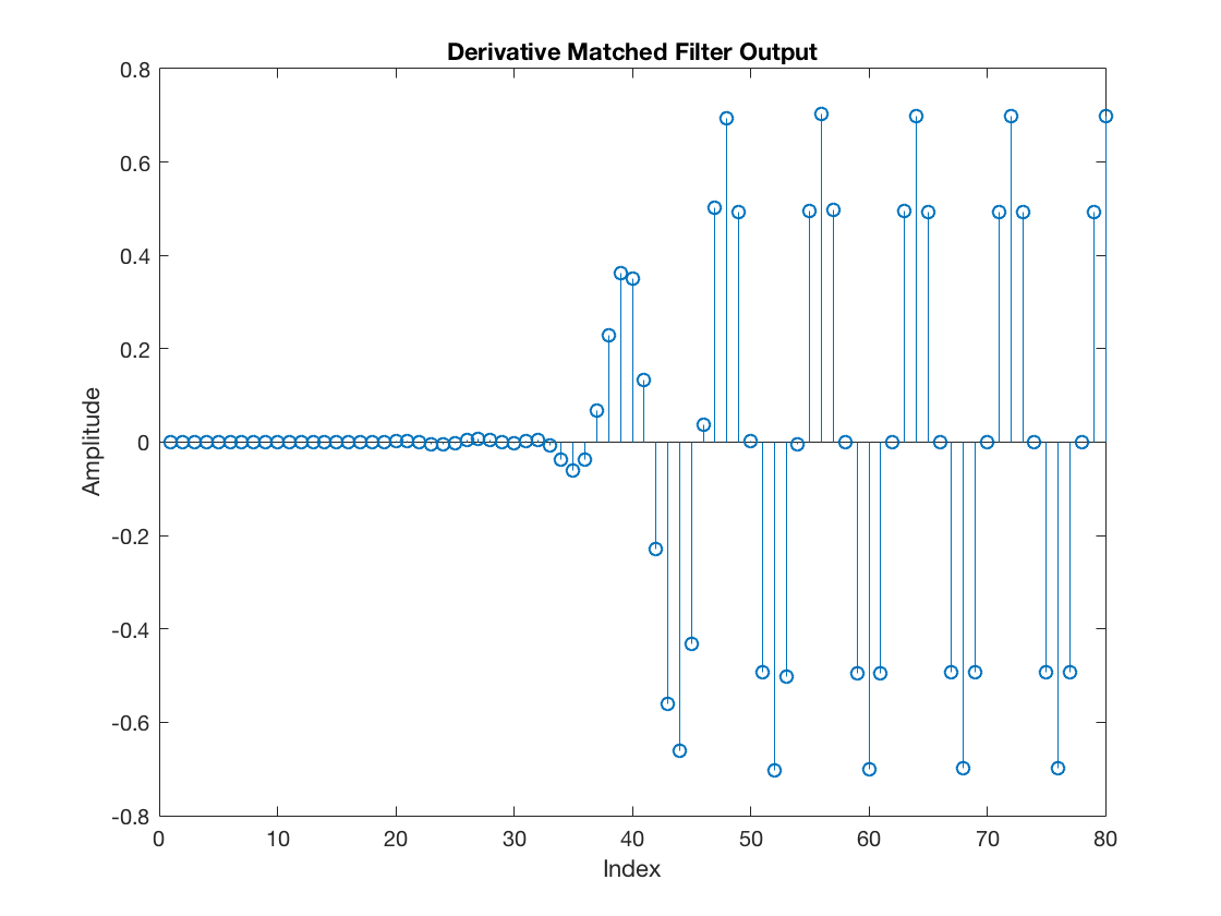
In the ML-TED scheme, the MF and dMF operate concurrently, filtering the same input sequence. Hence, continuing with the example, the dMF output looks as follows:
dmfOutput = filter(dmf, 1, rxDelayed);

figure
stem(dmfOutput)
title('Derivative Matched Filter Output')
xlabel('Index')
ylabel('Amplitude')
Furthermore, the ML-TED extracts a timing error precisely at the same instant when a sample from the MF output is retained as a symbol. The result is shown next. In particular, we can contrast the two scenarios discussed earlier, i.e., when the receiver is unaware of the symbol timing offset and the opposite case when it does know the correct timing offset.
dmfDownsampled_nosync = downsample(dmfOutput, L);
dmfDownsampled_withsync = downsample(dmfOutput, L, timeOffset);

figure
stem(dmfDownsampled_nosync)
hold on
stem(dmfDownsampled_withsync, '--r', 'LineWidth', 2)
xlabel('Symbol Index')
ylabel('Amplitude')
legend('No Symbol Timing Sync', 'With Sync')
title('Downsampled dMF output')
hold off
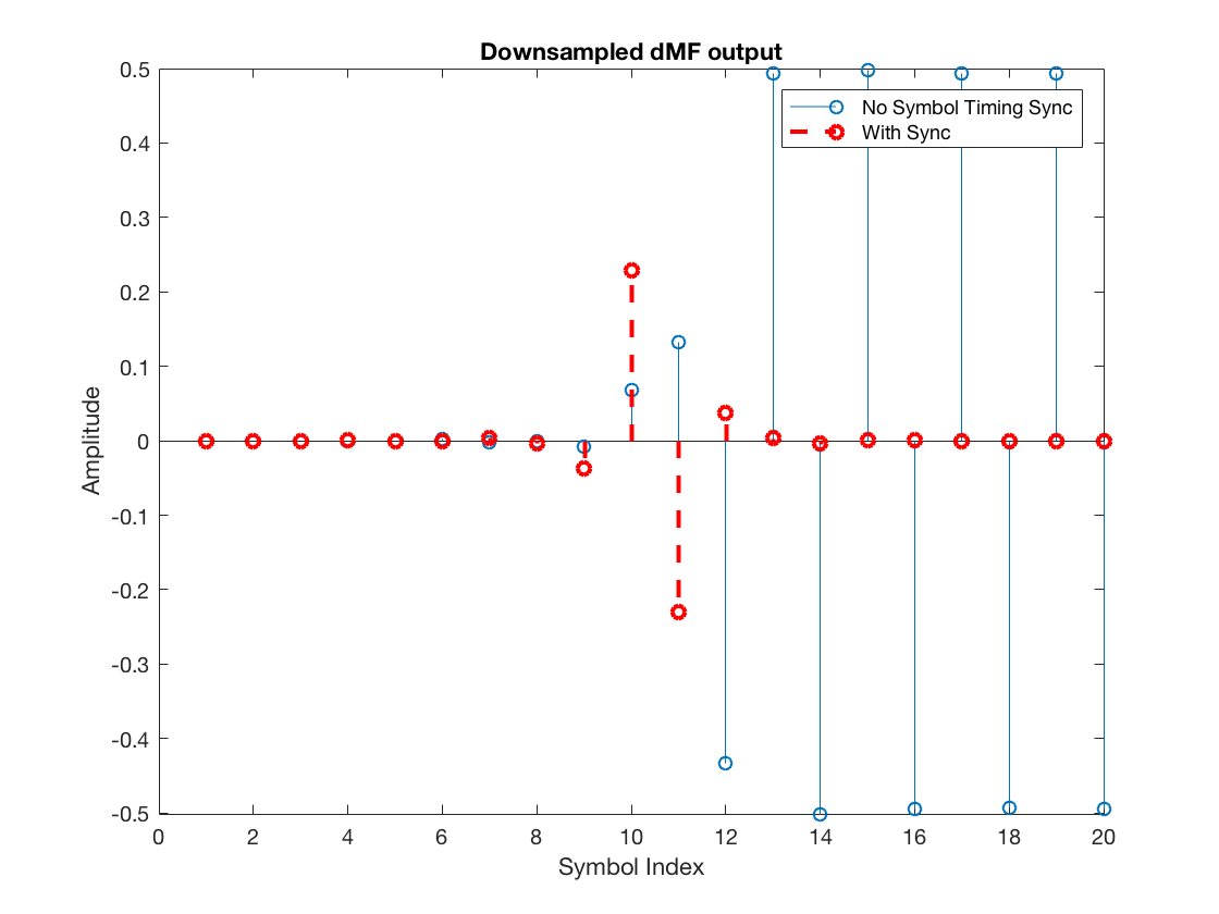
Note that the timing error metric output by the dMF has significant amplitude for the unsynchronized receiver but is practically null for the receiver that already knows the symbol timing offset. Hence, we can conclude that this dMF can be very useful. It will indicate the alignment (or misalignment) relative to the pulse shaping function’s peak and zero-crossings.
Nonetheless, note this particular ML-TED scheme has only worked above because we forced the transmit symbols to be continuously alternating between +1 and -1. When that is not true, as is the case for most practical random symbol streams, the ML-TED output can be very noisy. This noise has a specific name in the symbol timing recovery parlance. It is called self-noise [1]. Other TED schemes, such as the zero-crossing TED (ZC-TED), do not suffer from this noise.
Before advancing into the ZC-TED, there is one final remark. The ML-TED timing error samples above are not complete. It does not suffice to extract the raw downsampled values of the dMF. A sign correction must be applied to these values. A comprehensive explanation is provided for Fig. 8.2.2 in [1], but let’s summarize the idea here.
The unsynchronized receiver can be interpreted as a receiver guessing a timing offset \(\hat{\tau} = 0\) in units of sample intervals. However, the actual timing offset is \(\tau = 1\), so the timing error is \(\tau_e = \tau – \hat{\tau} = 1\). The solution is to increase the guess \(\hat{\tau}\) until obtaining a zero error (\(\tau_e = 0\)).
When the MF output is transitioning from a -1 symbol to a +1 symbol, the slope of the output is positive. In this case, if we extract a sample from the dMF output using \(\hat{\tau} = 0\), we get a positive value, which tells the receiver’s timing recovery loop that the current guess \(\hat{\tau}\) must be increased (because the error is positive). Such a positive error indication would be appropriate in the above example, where we need to increase the initial guess \(\hat{\tau} = 0\) to get closer to the true offset \(\tau = 1\). In contrast, when the MF output is transitioning from a +1 to -1, the slope of the MF output is negative, so the extracted dMF sample is negative. This negative value indicates the current guess \(\hat{\tau}\) must be decreased. That would drive the loop away from the true timing offset, which would be undesirable. Hence, we need some solution to obtain a correct error indication regardless of the underlying symbol transition.
Fortunately, there is a simple trick. If we multiply the dMF output by the detected symbol, note it would be multiplied by +1 in the positive transition (from -1 to +1, because -1 is the previous symbol and +1 is the current symbol) and multiplied by -1 in the negative transition (from +1 to -1). Thus, when the dMF has a negative slope (transition from +1 to -1), the dMF sample is multiplied by a negative value (symbol -1), compensating the slope sign.
Of course, because \(\tau\) is between 0 and L-1, the guess \(\hat{\tau}\) must be modulo-L. So, for example, if it is currently \(\hat{\tau} = 0\), and \(L = 4\), a unitary decrease would lead to \(\hat{\tau} = 3\).
Once sign correction (using the detected symbols) is applied, the following result is obtained:
% Detected Symbols

% First do PAM demodulation
rxdata_nosync   = pamdemod(downsample(mfOutput, L), M);
rxdata_withsync = pamdemod(downsample(mfOutput, L, timeOffset), M);
% Then, regenerate the corresponding constellation symbols
decSym_nosync   = real(pammod(rxdata_nosync, M));
decSym_withsync = real(pammod(rxdata_withsync, M));

% TED Output
e_nosync   = decSym_nosync .* dmfDownsampled_nosync;
e_withsync = decSym_withsync .* dmfDownsampled_withsync;

figure
stem(e_nosync)
hold on
stem(e_withsync, '--r', 'LineWidth', 2)
xlabel('Symbol Index')
ylabel('Amplitude')
legend('No Symbol Timing Sync', 'With Sync')
title('ML-TED Output - Timing Errors')
hold off
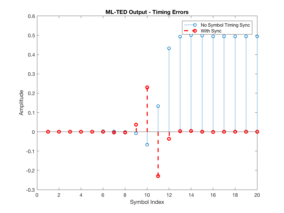
Observe that the TED output for the unsynchronized system is all positive after the RC pulse delay (of 10 symbols), which is the expected result given that the current guess \(\hat{\tau} = 0\) must be increased to approach the actual \(\tau = 1\).
Zero-crossing Timing Error Detector (ZC-TED)
Next, let’s investigate the ZC-TED, which, as stated earlier, has the advantage of avoiding self noise.
The principle exploited by the ZC-TED is that when the MF output transitions from +1 to -1 or vice versa, it crosses the zero amplitude. In particular, because there are L-1 samples between every two consecutive symbols, the zero-crossing is expected to lie near (if not precisely in) the middle index between these L-1 samples. Therefore, the receiver can constantly observe the sample at the midpoint between a transition and use this value as the timing error. Once the midpoint sample aligns with the zero-crossing, the error becomes zero, and the symbol timing recovery loop can converge (lock). If the midpoint sample is not zero, the current guess \(\hat{\tau}\) of the symbol timing offset must be adjusted.
Note that, with this mechanism, the ZC-TED scheme does not require a dMF filter at all. Instead, it operates solely by using the samples of the regular MF output. Hence, the ZC-TED can be implemented more efficiently than the ML-TED, avoiding the computational cost associated with the dMF filtering.
To understand the adjustment applied to the current guess \(\hat{\tau}\), we consider the two possible scenarios, a positive transition (from -1 to +1) and a negative transition (from +1 to -1). The plot below zooms into a negative transition observed on the unsynchronized system, namely the system whose current timing offset guess is \(\hat{\tau} = 0\).
figure
stem(mfOutput(41:41+L))
hold on
plot(mfOutput(41:41+L))
hold off
xlabel('Index')
ylabel('Amplitude')
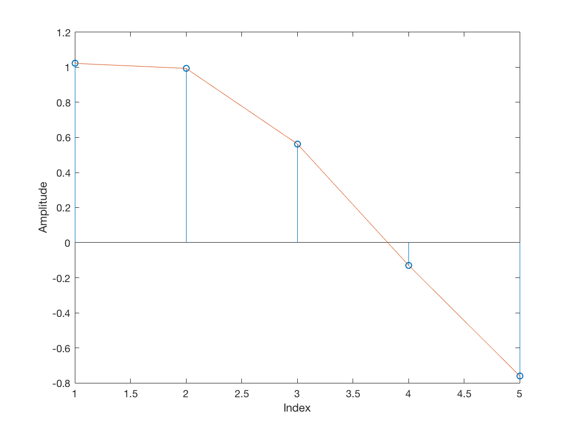
Note the midpoint sample (at index 3) is positive. Meanwhile, a positive transition (from -1 to +1) looks as follows:
figure
stem(mfOutput(45:45+L))
hold on
plot(mfOutput(45:45+L))
hold off
xlabel('Index')
ylabel('Amplitude')
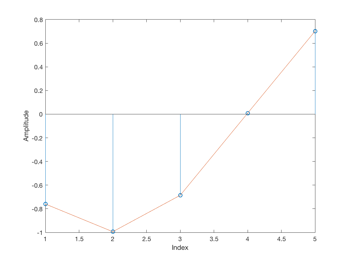
That is, the midpoint sample is negative. Hence, just like the ML-TED, the ZC-TED also needs a sign correction step. In both cases plotted above, the correct timing error indication should be a positive value, given that the current timing offset guess \(\hat{\tau} = 0\) must be increased to approach the actual \(\tau = 1\). However, the value observed on a positive transition was negative.
The proper way of sign-correcting the midpoint samples observed by the ZC-TED is by multiplication with the difference \(\hat{a}(k-1) – \hat{a}(k)\) between the previous and the current symbols. This difference can be based on the actual symbols when known at the receiver side (data-aided approach) or on decisions (decision-directed method).
Next, we can observe the sign-corrected ZC-TED output for the unsynchronized and perfectly synchronized systems:
% Midpoint samples
midSamples_nosync   = mfOutput((L/2 + 1):L:end);
midSamples_withsync = mfOutput((L/2 + 1 + timeOffset):L:end);

% Sign correction values based on symbol decisions:
signcorrection_nosync   = [-diff(decSym_nosync), 0];
signcorrection_withsync = [-diff(decSym_withsync), 0];
% Note: the padded zero is just for the signcorrection vector
% to have a length equivalent to the the vector of midsamples.

% ZC-TED output:
zcted_nosync   = midSamples_nosync .* signcorrection_nosync;
zcted_withsync = midSamples_withsync .* signcorrection_withsync;

% Plot
figure
stem(zcted_nosync)
hold on
stem(zcted_withsync, '--r', 'LineWidth', 2)
hold off
xlabel('Symbol Index')
ylabel('Amplitude')
legend('No Symbol Timing Sync', 'With Sync')
title('ZC-TED Output - Timing Errors')
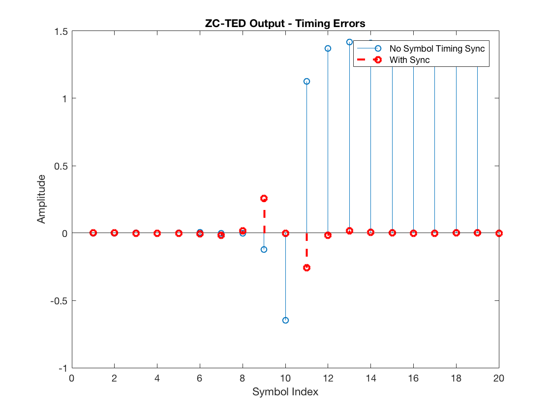
Note the ZC-TED yields reasonable timing error indication. Namely, it outputs positive timing error values for the unsynchronized receiver (again, after the RC pulse delay) and zero values for the perfectly synchronized receiver.
Finally, observe the reason why the ZC-TED scheme does not suffer from self noise. It is because the sign-correction term \(\hat{a}(k-1) – \hat{a}(k)\) is \(0\) when two consecutive symbols are equal, i.e., +1 and +1, or -1 and -1. As a result, the scheme does not request any timing correction when there is no zero-crossing between two symbols. In contrast, with the ML-TED, even though it requires a data transition to yield a reasonable timing error estimate, it does not eliminate the timing error estimate when the consecutive symbols are equal, leading to self noise.
Final Remarks
This tutorial provided an introduction to the concept of symbol timing synchronization. If you are interested in digging deeper into the topic, I suggest experimenting with the simulator and scripts available on the Symbol Timing Sync Github repository. The simulator implements a complete timing recovery loop, including a PI controller, an interpolator (with multiple options), and an interpolation control scheme based on the modulo-1 counter explained in [1]. Furthermore, the simulator includes useful debugging features, such as a time scope to show relevant loop metrics in “in real-time” (evolving over the simulation). Feel free to experiment with it and even contribute to the repository.
References
[1] Rice, Michael. Digital Communications: A Discrete-Time Approach. Upper Saddle River, NJ: Prentice Hall, 2009.
Leave a Reply